

The new geoip2 parser of syslog-ng 3.11 is not only faster than its predecessor, but can also provide a lot more detailed geographical information about IP addresses. Next to the usual country name and longitude/latitude information, it also provides the continent, time zone, postal code and even county name. Some of these are available in multiple languages. Learn how you can utilize this information by parsing logs from iptables using syslog-ng, storing them to Elasticsearch, and displaying the results in Kibana!
Before you begin
First of all, you need some iptables log messages. In my case, I used logs from my Turris Omnia router. You could use logs from another device running iptables. Alternatively, with a small effort, you can replace iptables with an Apache web server or any other application that saves IP addresses as part of its log message.
You will also need a syslog-ng version that has the new geoip2 parser. The new geoip2 parser was released as part of version 3.11.1.
As syslog-ng packages in Linux distributions do not include the Elasticsearch destination of syslog-ng, you either need to compile it yourself or use one of the unofficial packages, as listed at https://www.syslog-ng.com/products/open-source-log-management/3rd-party-binaries.aspx.
Last but not least, you will also need Elasticsearch and Kibana installed. I used version 5.5.1 of the Elastic stack, but any other version should work just fine.
What is new in GeoIP
The geoip2 parser of syslog-ng uses the maxminddb library to look up geographical information. It is considerably faster than its predecessor and also provides a lot more detailed information.
As usual, the packaging of maxminddb tools is different on different Linux distributions. You need to make sure that a tool to download / update database files is installed, together with the mmdblookup tool. On most distributions you need to use the former at least once as usually only the old type of databases are available packaged. The latter application can help you list what kind of information is available in the database.
Here is a shortened example:
[root@localhost-czp ~]# mmdblookup --file /usr/share/GeoIP/GeoLite2-City.mmdb --ip 1.2.3.4

  {
    "city":
      {
        "geoname_id":
          3054643 <uint32>
        "names":
          {
            "de":
              "Budapest" <utf8_string>
            "en":
              "Budapest" <utf8_string>
            "es":
              "Budapest" <utf8_string>
            "fr":
              "Budapest" <utf8_string>
            "ja":
              "ブダペスト" <utf8_string>
            "pt-BR":
              "Budapeste" <utf8_string>
            "ru":
              "Будапешт" <utf8_string>
            "zh-CN":
              "布达佩斯" <utf8_string>
          }
      }
[...]
    "location":
      {
        "accuracy_radius":
          100 <uint16>
        "latitude":
          47.500000 <double>
        "longitude":
          19.083300 <double>
        "time_zone":
          "Europe/Budapest" <utf8_string>
      }
[...]
As you can see from the above command line, I use the freely available GeoLite2-City database. The commercial variant is also supported by syslog-ng, which is more precise and up-to-date.
In my configuration example below, I chose to simply store all available geographical data, but normally that is a waste of resources. You can figure out the hierarchy of names based on the JSON output of mmdblookup.
Configure Elasticsearch
The installation and configuration of Elasticsearch and Kibana are beyond the scope of this blog. The only thing I want to note here is that before sending logs from syslog-ng to Elasticsearch, you have to configure mapping for geo information.
If you follow my configuration examples below, you can use the following mapping. I use “syslog-ng” as the index name.
{
   "mappings" : {
      "_default_" : {
         "properties" : {
            "geoip2" : {
               "properties" : {
                  "location2" : {
                     "type" : "geo_point"
                  }
               }
            }
         }
      }
   }
}
Complete these steps to get your syslog-ng ready for creating heat maps:
1. First of all, you need some logs. In my test environment I receive iptables logs from my router over a TCP connection to port 514. These are filtered on the sender side, so no other logs are included. If you do not have filtered logs, in most cases you can filter for firewall logs based on the program name.
source s_tcp {
  tcp(ip("0.0.0.0") port("514"));
};
2. Process log messages. The first step of processing is using the key-value parser. It creates name-value pairs from the content of the message. You can store all or part of these name-value pairs in a database and search them at a field level instead of the whole message. A prefix for the name is used to make sure that the names do not overlap.
parser p_kv {kv-parser(prefix("kv.")); };
The source IP of the attacker is stored into the kv.SRC name-value pair.
3. Let’s analyze the kv.SRC name-value pair further, using the geoip2 parser. As usual, we use a prefix to avoid any naming problems. Note that the location of the database might be different on your system.
parser p_geoip2 { geoip2( "${kv.SRC}", prefix( "geoip2." ) database( "/usr/share/GeoIP/GeoLite2-City.mmdb" ) ); };
4. The next step is necessary to ensure that location information is in the form expected by Elasticsearch. It looks slightly more complicated than for the first version of the GeoIP parser as there is more information available and information is now structured.
rewrite r_geoip2 {
    set(
        "${geoip2.location.latitude},${geoip2.location.longitude}",
        value( "geoip2.location2" ),
        condition(not "${geoip2.location.latitude}" == "")
    );
};
5. In the Elasticsearch destination we assume that both the cluster and index names are “syslog-ng”. We set the flush-limit to a low value as we do not expect a high message rate. A low flush-limit makes sure that we see logs in Kibana in near real-time. By default, it is set to a much higher value, which is perfect for performance. Unfortunately, timeout is not implemented in the Java destinations so with the default setting and low message rate, you might need to wait an hour before anything shows up in Elasticsearch.
destination d_elastic {
 elasticsearch2 (
  cluster("syslog-ng")
  client-mode("http")
  index("syslog-ng")
  type("test")
  flush-limit("1")
  template("$(format-json --scope rfc5424 --scope nv-pairs --exclude DATE --key ISODATE)")
 )
};
6. Finally we need a log statement which connects all of these building blocks together:
log {
  source(s_tcp);
  parser(p_kv);
  parser(p_geoip2);
  rewrite(r_geoip2);
  destination(d_elastic);
};
Configuration to copy & paste
To make your life easier, I compiled these configuration snippets in one place for better copy & paste experience. You should append it to your syslog-ng.conf or place it in a separate .conf file under /etc/syslog-ng/conf.d/ − if supported by your Linux distribution.
source s_tcp {
  tcp(ip("0.0.0.0") port("514"));
};

parser p_kv {kv-parser(prefix("kv.")); };

parser p_geoip2 { geoip2( "${kv.SRC}", prefix( "geoip2." ) database( "/usr/share/GeoIP/GeoLite2-City.mmdb" ) ); };

rewrite r_geoip2 {
    set(
        "${geoip2.location.latitude},${geoip2.location.longitude}",
        value( "geoip2.location2" ),
        condition(not "${geoip2.location.latitude}" == "")
    );
};

destination d_elastic {
 elasticsearch2 (
  cluster("syslog-ng")
  client-mode("http")
  index("syslog-ng")
  type("test")
  flush-limit("1")
  template("$(format-json --scope rfc5424 --scope nv-pairs --exclude DATE --key ISODATE)")
 )
};

log {
  source(s_tcp);
  parser(p_kv);
  parser(p_geoip2);
  rewrite(r_geoip2);
  destination(d_elastic);
};
Visualize your data
By now you have configured syslog-ng to parse iptables logs, added geographical information to them, and stored the results in Elasticsearch. The next step is to verify if logs arrive to Elasticsearch. You should see messages in Kibana where many field names start with “kv.” and “geoip2.”
Once you verified that logs are arriving to Elasticsearch, you can start creating some visualizations. There are numerous tutorials on how to do it by Elastic and others.
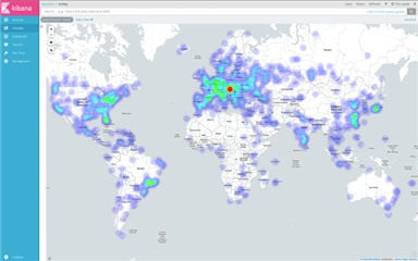
You can see a world map below visualizing the IP addresses that attempt to connect to my router. You can easily create such a map just by clicking on the “geoip2.location2” field in the “Available fields” list in Kibana, and then clicking on the “Visualize” button when it appears below the field name.
Even if I left out many details, this blog is now quite lengthy so I am going to point you to some further reading: